1.5.12.17. Plotting and manipulating FFTs for filtering

Plot the power of the FFT of a signal and inverse FFT back to reconstruct a signal.

This example demonstrate scipy.fftpack.fft(), scipy.fftpack.fftfreq() and scipy.fftpack.ifft(). It implements a basic filter that is very suboptimal, and should not be used.

import numpy as np
import scipy as sp
import matplotlib.pyplot as plt

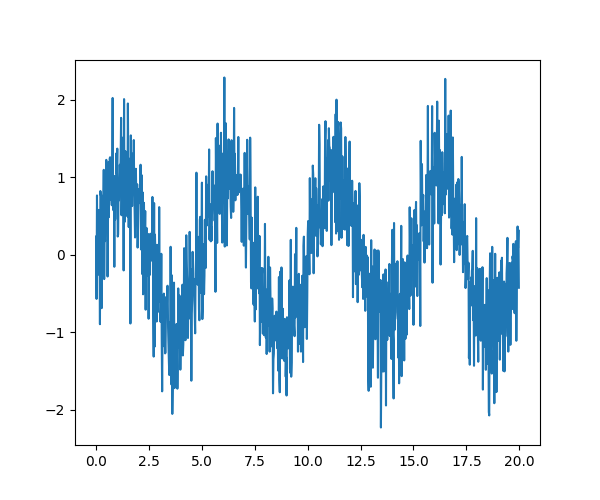
Generate the signal

# Seed the random number generator
np.random.seed(1234)

time_step = 0.02
period = 5.

time_vec = np.arange(0, 20, time_step)
sig = (np.sin(2 * np.pi / period * time_vec)
       + 0.5 * np.random.randn(time_vec.size))

plt.figure(figsize=(6, 5))
plt.plot(time_vec, sig, label='Original signal')

[<matplotlib.lines.Line2D object at 0x7fe7b0790160>]

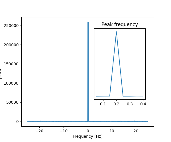
Compute and plot the power

# The FFT of the signal
sig_fft = sp.fftpack.fft(sig)

# And the power (sig_fft is of complex dtype)
power = np.abs(sig_fft)**2

# The corresponding frequencies
sample_freq = sp.fftpack.fftfreq(sig.size, d=time_step)

# Plot the FFT power
plt.figure(figsize=(6, 5))
plt.plot(sample_freq, power)
plt.xlabel('Frequency [Hz]')
plt.ylabel('plower')

# Find the peak frequency: we can focus on only the positive frequencies
pos_mask = np.where(sample_freq > 0)
freqs = sample_freq[pos_mask]
peak_freq = freqs[power[pos_mask].argmax()]

# Check that it does indeed correspond to the frequency that we generate
# the signal with
np.allclose(peak_freq, 1./period)

# An inner plot to show the peak frequency
axes = plt.axes([0.55, 0.3, 0.3, 0.5])
plt.title('Peak frequency')
plt.plot(freqs[:8], power[pos_mask][:8])
plt.setp(axes, yticks=[])

# scipy.signal.find_peaks_cwt can also be used for more advanced
# peak detection

[]

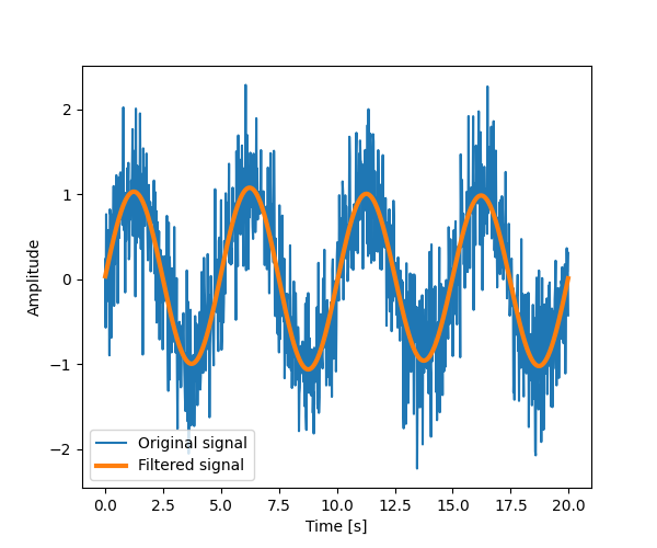
Remove all the high frequencies

We now remove all the high frequencies and transform back from frequencies to signal.

high_freq_fft = sig_fft.copy()
high_freq_fft[np.abs(sample_freq) > peak_freq] = 0
filtered_sig = sp.fftpack.ifft(high_freq_fft)

plt.figure(figsize=(6, 5))
plt.plot(time_vec, sig, label='Original signal')
plt.plot(time_vec, filtered_sig, linewidth=3, label='Filtered signal')
plt.xlabel('Time [s]')
plt.ylabel('Amplitude')

plt.legend(loc='best')

/opt/buildhome/python3.8/lib/python3.8/site-packages/matplotlib/cbook/__init__.py:1335: ComplexWarning: Casting complex values to real discards the imaginary part
  return np.asarray(x, float)

<matplotlib.legend.Legend object at 0x7fe7b042c100>

Note This is actually a bad way of creating a filter: such brutal cut-off in frequency space does not control distorsion on the signal.

Filters should be created using the SciPy filter design code

plt.show()