3.3. Scikit-image: image processing

Author: Emmanuelle Gouillart

scikit-image is a Python package dedicated to image processing, and using natively NumPy arrays as image objects. This chapter describes how to use scikit-image on various image processing tasks, and insists on the link with other scientific Python modules such as NumPy and SciPy.

See also

For basic image manipulation, such as image cropping or simple filtering, a large number of simple operations can be realized with NumPy and SciPy only. See Image manipulation and processing using NumPy and SciPy.

Note that you should be familiar with the content of the previous chapter before reading the current one, as basic operations such as masking and labeling are a prerequisite.

3.3.1. Introduction and concepts

Images are NumPy’s arrays np.ndarray

image:

np.ndarray

pixels:

array values: a[2, 3]

channels:

array dimensions

image encoding:

dtype (np.uint8, np.uint16, np.float)

filters:

functions (numpy, skimage, scipy)

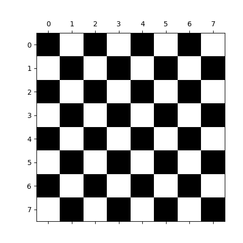
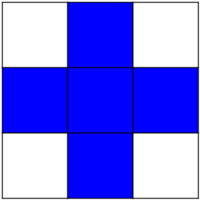
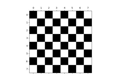
>>> import numpy as np
>>> check = np.zeros((8, 8))
>>> check[::2, 1::2] = 1
>>> check[1::2, ::2] = 1
>>> import matplotlib.pyplot as plt
>>> plt.imshow(check, cmap='gray', interpolation='nearest') 

3.3.1.1. scikit-image and the SciPy ecosystem

Recent versions of scikit-image is packaged in most scientific Python distributions, such as Anaconda or Enthought Canopy. It is also packaged for Ubuntu/Debian.

>>> import skimage
>>> from skimage import data  # most functions are in subpackages

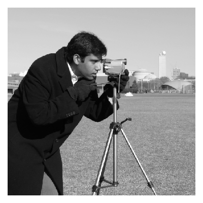
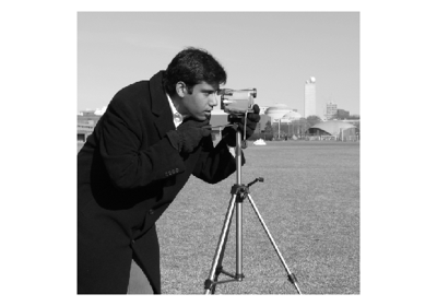
Most scikit-image functions take NumPy ndarrays as arguments

>>> camera = data.camera()
>>> camera.dtype
dtype('uint8')
>>> camera.shape
(512, 512)
>>> from skimage import filters
>>> filtered_camera = filters.gaussian(camera, 1)
>>> type(filtered_camera)   
<type 'numpy.ndarray'>

Other Python packages are available for image processing and work with NumPy arrays:

• scipy.ndimage : for nd-arrays. Basic filtering, mathematical morphology, regions properties

• Mahotas

Also, powerful image processing libraries have Python bindings:

• OpenCV (computer vision)

• ITK (3D images and registration)

• and many others

(but they are less Pythonic and NumPy friendly, to a variable extent).

3.3.1.2. What’s to be found in scikit-image

• Website: https://scikit-image.org/

• Gallery of examples: https://scikit-image.org/docs/stable/auto_examples/

Different kinds of functions, from boilerplate utility functions to high-level recent algorithms.

• Filters: functions transforming images into other images.

  • NumPy machinery

  • Common filtering algorithms

• Data reduction functions: computation of image histogram, position of local maxima, of corners, etc.

• Other actions: I/O, visualization, etc.

3.3.2. Input/output, data types and colorspaces

I/O: skimage.io

>>> from skimage import io

Reading from files: skimage.io.imread()

>>> import os
>>> filename = os.path.join(skimage.data_dir, 'camera.png')
>>> camera = io.imread(filename) 

Works with all data formats supported by the Python Imaging Library (or any other I/O plugin provided to imread with the plugin keyword argument).

Also works with URL image paths:

>>> logo = io.imread('https://scikit-image.org/_static/img/logo.png')

Saving to files:

>>> io.imsave('local_logo.png', logo)

(imsave also uses an external plugin such as PIL)

3.3.2.1. Data types

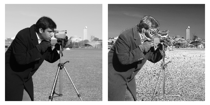
Image ndarrays can be represented either by integers (signed or unsigned) or floats.

Careful with overflows with integer data types

>>> camera = data.camera()
>>> camera.dtype
dtype('uint8')
>>> camera_multiply = 3 * camera

Different integer sizes are possible: 8-, 16- or 32-bytes, signed or unsigned.

Warning

An important (if questionable) skimage convention: float images are supposed to lie in [-1, 1] (in order to have comparable contrast for all float images)

>>> from skimage import img_as_float
>>> camera_float = img_as_float(camera)
>>> camera.max(), camera_float.max()
(255, 1.0)

Some image processing routines need to work with float arrays, and may hence output an array with a different type and the data range from the input array

>>> from skimage import filters
>>> camera_sobel = filters.sobel(camera)
>>> camera_sobel.max() 
0.591502...

Utility functions are provided in skimage to convert both the dtype and the data range, following skimage’s conventions: util.img_as_float, util.img_as_ubyte, etc.

See the user guide for more details.

3.3.2.2. Colorspaces

Color images are of shape (N, M, 3) or (N, M, 4) (when an alpha channel encodes transparency)

>>> face = sp.datasets.face()
>>> face.shape
(768, 1024, 3)

Routines converting between different colorspaces (RGB, HSV, LAB etc.) are available in skimage.color : color.rgb2hsv, color.lab2rgb, etc. Check the docstring for the expected dtype (and data range) of input images.

3D images

Most functions of skimage can take 3D images as input arguments. Check the docstring to know if a function can be used on 3D images (for example MRI or CT images).

Exercise

Open a color image on your disk as a NumPy array.

Find a skimage function computing the histogram of an image and plot the histogram of each color channel

Convert the image to grayscale and plot its histogram.

3.3.3. Image preprocessing / enhancement

Goals: denoising, feature (edges) extraction, …

3.3.3.1. Local filters

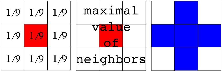
Local filters replace the value of pixels by a function of the values of neighboring pixels. The function can be linear or non-linear.

Neighbourhood: square (choose size), disk, or more complicated structuring element.

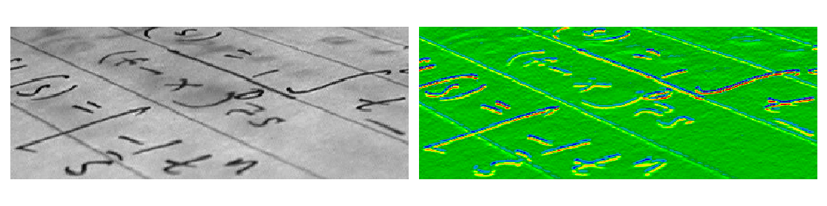
Example : horizontal Sobel filter

>>> text = data.text()
>>> hsobel_text = filters.sobel_h(text)

Uses the following linear kernel for computing horizontal gradients:

1   2   1
0   0   0
-1  -2  -1

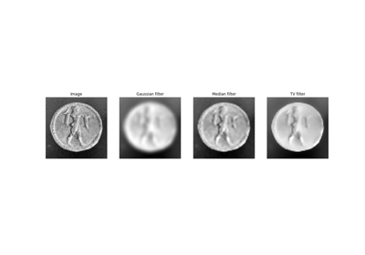
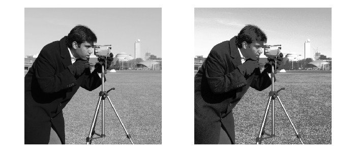
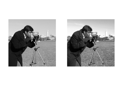
3.3.3.2. Non-local filters

Non-local filters use a large region of the image (or all the image) to transform the value of one pixel:

>>> from skimage import exposure
>>> camera = data.camera()
>>> camera_equalized = exposure.equalize_hist(camera)

Enhances contrast in large almost uniform regions.

3.3.3.3. Mathematical morphology

See wikipedia for an introduction on mathematical morphology.

Probe an image with a simple shape (a structuring element), and modify this image according to how the shape locally fits or misses the image.

Default structuring element: 4-connectivity of a pixel

>>> from skimage import morphology
>>> morphology.diamond(1)
array([[0, 1, 0],
       [1, 1, 1],
       [0, 1, 0]], dtype=uint8)

Erosion = minimum filter. Replace the value of a pixel by the minimal value covered by the structuring element.:

>>> a = np.zeros((7,7), dtype=np.uint8)
>>> a[1:6, 2:5] = 1
>>> a
array([[0, 0, 0, 0, 0, 0, 0],
       [0, 0, 1, 1, 1, 0, 0],
       [0, 0, 1, 1, 1, 0, 0],
       [0, 0, 1, 1, 1, 0, 0],
       [0, 0, 1, 1, 1, 0, 0],
       [0, 0, 1, 1, 1, 0, 0],
       [0, 0, 0, 0, 0, 0, 0]], dtype=uint8)
>>> morphology.binary_erosion(a, morphology.diamond(1)).astype(np.uint8)
array([[0, 0, 0, 0, 0, 0, 0],
       [0, 0, 0, 0, 0, 0, 0],
       [0, 0, 0, 1, 0, 0, 0],
       [0, 0, 0, 1, 0, 0, 0],
       [0, 0, 0, 1, 0, 0, 0],
       [0, 0, 0, 0, 0, 0, 0],
       [0, 0, 0, 0, 0, 0, 0]], dtype=uint8)
>>> #Erosion removes objects smaller than the structure
>>> morphology.binary_erosion(a, morphology.diamond(2)).astype(np.uint8)
array([[0, 0, 0, 0, 0, 0, 0],
       [0, 0, 0, 0, 0, 0, 0],
       [0, 0, 0, 0, 0, 0, 0],
       [0, 0, 0, 0, 0, 0, 0],
       [0, 0, 0, 0, 0, 0, 0],
       [0, 0, 0, 0, 0, 0, 0],
       [0, 0, 0, 0, 0, 0, 0]], dtype=uint8)

Dilation: maximum filter:

>>> a = np.zeros((5, 5))
>>> a[2, 2] = 1
>>> a
array([[0.,  0.,  0.,  0.,  0.],
       [0.,  0.,  0.,  0.,  0.],
       [0.,  0.,  1.,  0.,  0.],
       [0.,  0.,  0.,  0.,  0.],
       [0.,  0.,  0.,  0.,  0.]])
>>> morphology.binary_dilation(a, morphology.diamond(1)).astype(np.uint8)
array([[0, 0, 0, 0, 0],
       [0, 0, 1, 0, 0],
       [0, 1, 1, 1, 0],
       [0, 0, 1, 0, 0],
       [0, 0, 0, 0, 0]], dtype=uint8)

Opening: erosion + dilation:

>>> a = np.zeros((5,5), dtype=int)
>>> a[1:4, 1:4] = 1; a[4, 4] = 1
>>> a
array([[0, 0, 0, 0, 0],
       [0, 1, 1, 1, 0],
       [0, 1, 1, 1, 0],
       [0, 1, 1, 1, 0],
       [0, 0, 0, 0, 1]])
>>> morphology.binary_opening(a, morphology.diamond(1)).astype(np.uint8)
array([[0, 0, 0, 0, 0],
       [0, 0, 1, 0, 0],
       [0, 1, 1, 1, 0],
       [0, 0, 1, 0, 0],
       [0, 0, 0, 0, 0]], dtype=uint8)

Opening removes small objects and smoothes corners.

Grayscale mathematical morphology

Mathematical morphology operations are also available for (non-binary) grayscale images (int or float type). Erosion and dilation correspond to minimum (resp. maximum) filters.

Higher-level mathematical morphology are available: tophat, skeletonization, etc.

See also

Basic mathematical morphology is also implemented in scipy.ndimage.morphology. The scipy.ndimage implementation works on arbitrary-dimensional arrays.

---

Example of filters comparison: image denoising

>>> from skimage.morphology import disk
>>> coins = data.coins()
>>> coins_zoom = coins[10:80, 300:370]
>>> median_coins = filters.median(coins_zoom, disk(1))
>>> from skimage import restoration
>>> tv_coins = restoration.denoise_tv_chambolle(coins_zoom, weight=0.1)
>>> gaussian_coins = filters.gaussian(coins, sigma=2)

3.3.4. Image segmentation

Image segmentation is the attribution of different labels to different regions of the image, for example in order to extract the pixels of an object of interest.

3.3.4.1. Binary segmentation: foreground + background

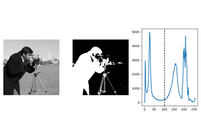
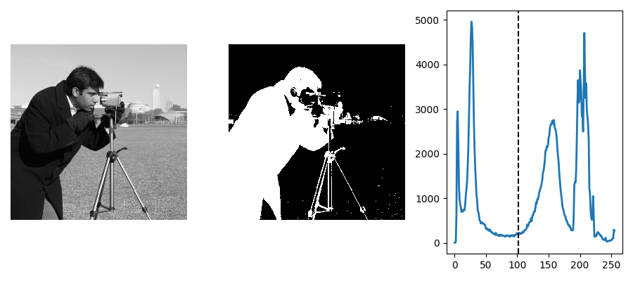
Histogram-based method: Otsu thresholding

Tip

The Otsu method is a simple heuristic to find a threshold to separate the foreground from the background.

Earlier scikit-image versions

skimage.filters is called skimage.filter in earlier versions of scikit-image

from skimage import data
from skimage import filters
camera = data.camera()
val = filters.threshold_otsu(camera)
mask = camera < val

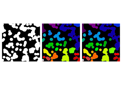
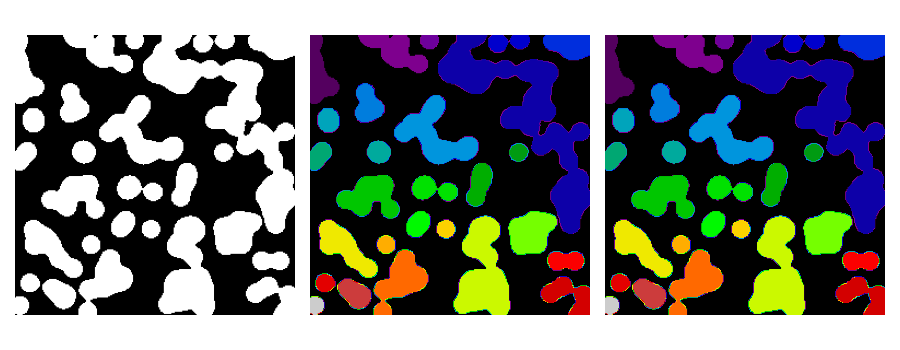
Labeling connected components of a discrete image

Tip

Once you have separated foreground objects, it is use to separate them from each other. For this, we can assign a different integer labels to each one.

Synthetic data:

>>> n = 20
>>> l = 256
>>> im = np.zeros((l, l))
>>> points = l * np.random.random((2, n ** 2))
>>> im[(points[0]).astype(int), (points[1]).astype(int)] = 1
>>> im = filters.gaussian(im, sigma=l / (4. * n))
>>> blobs = im > im.mean()

Label all connected components:

>>> from skimage import measure
>>> all_labels = measure.label(blobs)

Label only foreground connected components:

>>> blobs_labels = measure.label(blobs, background=0)

See also

scipy.ndimage.find_objects() is useful to return slices on object in an image.

3.3.4.2. Marker based methods

If you have markers inside a set of regions, you can use these to segment the regions.

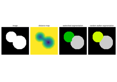
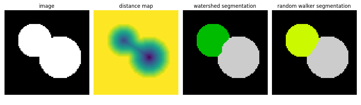
Watershed segmentation

The Watershed (skimage.segmentation.watershed()) is a region-growing approach that fills “basins” in the image

>>> from skimage import morphology
>>> from skimage.segmentation import watershed
>>> from skimage.feature import peak_local_max
>>>
>>> # Generate an initial image with two overlapping circles
>>> x, y = np.indices((80, 80))
>>> x1, y1, x2, y2 = 28, 28, 44, 52
>>> r1, r2 = 16, 20
>>> mask_circle1 = (x - x1) ** 2 + (y - y1) ** 2 < r1 ** 2
>>> mask_circle2 = (x - x2) ** 2 + (y - y2) ** 2 < r2 ** 2
>>> image = np.logical_or(mask_circle1, mask_circle2)
>>> # Now we want to separate the two objects in image
>>> # Generate the markers as local maxima of the distance
>>> # to the background
>>> import scipy as sp
>>> distance = sp.ndimage.distance_transform_edt(image)
>>> peak_idx = peak_local_max(distance, footprint=np.ones((3, 3)), labels=image)
>>> peak_mask = np.zeros_like(distance, dtype=bool)
>>> peak_mask[tuple(peak_idx.T)] = True
>>> markers = morphology.label(peak_mask)
>>> labels_ws = watershed(-distance, markers, mask=image)

Random walker segmentation

The random walker algorithm (skimage.segmentation.random_walker()) is similar to the Watershed, but with a more “probabilistic” approach. It is based on the idea of the diffusion of labels in the image:

>>> from skimage import segmentation
>>> # Transform markers image so that 0-valued pixels are to
>>> # be labelled, and -1-valued pixels represent background
>>> markers[~image] = -1
>>> labels_rw = segmentation.random_walker(image, markers)

Postprocessing label images

skimage provides several utility functions that can be used on label images (ie images where different discrete values identify different regions). Functions names are often self-explaining: skimage.segmentation.clear_border(), skimage.segmentation.relabel_from_one(), skimage.morphology.remove_small_objects(), etc.

Exercise

• Load the coins image from the data submodule.

• Separate the coins from the background by testing several segmentation methods: Otsu thresholding, adaptive thresholding, and watershed or random walker segmentation.

• If necessary, use a postprocessing function to improve the coins / background segmentation.

3.3.5. Measuring regions’ properties

>>> from skimage import measure

Example: compute the size and perimeter of the two segmented regions:

>>> properties = measure.regionprops(labels_rw)
>>> [float(prop.area) for prop in properties]
[770.0, 1168.0]
>>> [prop.perimeter for prop in properties] 
[100.91..., 126.81...]

See also

for some properties, functions are available as well in scipy.ndimage.measurements with a different API (a list is returned).

Exercise (continued)

• Use the binary image of the coins and background from the previous exercise.

• Compute an image of labels for the different coins.

• Compute the size and eccentricity of all coins.

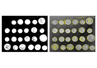
3.3.6. Data visualization and interaction

Meaningful visualizations are useful when testing a given processing pipeline.

Some image processing operations:

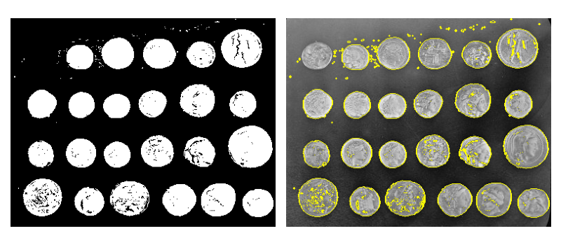
>>> coins = data.coins()
>>> mask = coins > filters.threshold_otsu(coins)
>>> clean_border = segmentation.clear_border(mask)

Visualize binary result:

>>> plt.figure() 
<Figure size ... with 0 Axes>
>>> plt.imshow(clean_border, cmap='gray') 
<matplotlib.image.AxesImage object at 0x...>

Visualize contour

>>> plt.figure() 
<Figure size ... with 0 Axes>
>>> plt.imshow(coins, cmap='gray') 
<matplotlib.image.AxesImage object at 0x...>
>>> plt.contour(clean_border, [0.5]) 
<matplotlib.contour.QuadContourSet ...>

Use skimage dedicated utility function:

>>> coins_edges = segmentation.mark_boundaries(coins, clean_border.astype(int))

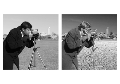
3.3.7. Feature extraction for computer vision

Geometric or textural descriptor can be extracted from images in order to

• classify parts of the image (e.g. sky vs. buildings)

• match parts of different images (e.g. for object detection)

• and many other applications of Computer Vision

>>> from skimage import feature

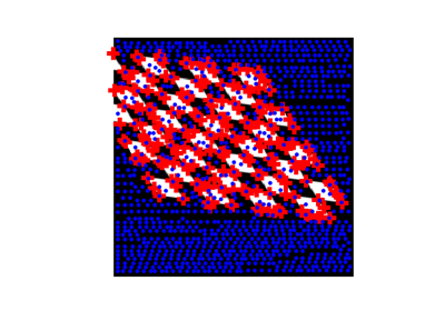
Example: detecting corners using Harris detector

from skimage.feature import corner_harris, corner_subpix, corner_peaks
from skimage.transform import warp, AffineTransform


tform = AffineTransform(scale=(1.3, 1.1), rotation=1, shear=0.7,
                        translation=(210, 50))
image = warp(data.checkerboard(), tform.inverse, output_shape=(350, 350))

coords = corner_peaks(corner_harris(image), min_distance=5)
coords_subpix = corner_subpix(image, coords, window_size=13)

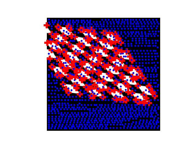
(this example is taken from the plot_corner example in scikit-image)

Points of interest such as corners can then be used to match objects in different images, as described in the plot_matching example of scikit-image.

3.3.8. Full code examples

3.3.9. Examples for the scikit-image chapter

Creating an image

Creating an image

Displaying a simple image

Displaying a simple image

Integers can overflow

Integers can overflow

Equalizing the histogram of an image

Equalizing the histogram of an image

Computing horizontal gradients with the Sobel filter

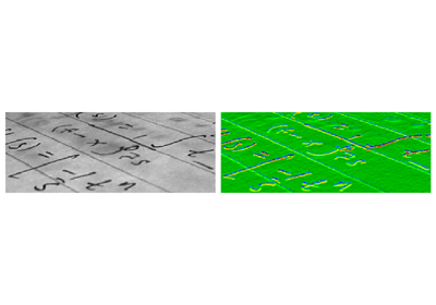
Computing horizontal gradients with the Sobel filter

Segmentation contours

Segmentation contours

Otsu thresholding

Otsu thresholding

Labelling connected components of an image

Labelling connected components of an image

Affine transform

Affine transform

Various denoising filters

Various denoising filters

Watershed and random walker for segmentation

Watershed and random walker for segmentation