2.7.4.10. Alternating optimization

The challenge here is that Hessian of the problem is a very ill-conditioned matrix. This can easily be seen, as the Hessian of the first term in simply 2 * K.T @ K. Thus the conditioning of the problem can be judged from looking at the conditioning of K.

import time

import numpy as np
import scipy as sp
import matplotlib.pyplot as plt

np.random.seed(0)

K = np.random.normal(size=(100, 100))

def f(x):
    return np.sum((K @ (x - 1))**2) + np.sum(x**2)**2


def f_prime(x):
    return 2 * K.T @ K @ (x - 1) + 4*np.sum(x**2)*x


def hessian(x):
    H = 2 * K.T @ K + 4*2*x*x[:, np.newaxis]
    return H + 4*np.eye(H.shape[0])*np.sum(x**2)

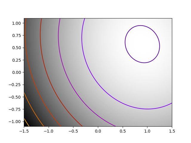
Some pretty plotting

plt.figure(1)
plt.clf()
Z = X, Y = np.mgrid[-1.5:1.5:100j, -1.1:1.1:100j]
# Complete in the additional dimensions with zeros
Z = np.reshape(Z, (2, -1)).copy()
Z.resize((100, Z.shape[-1]))
Z = np.apply_along_axis(f, 0, Z)
Z = np.reshape(Z, X.shape)
plt.imshow(Z.T, cmap=plt.cm.gray_r, extent=[-1.5, 1.5, -1.1, 1.1],
          origin='lower')
plt.contour(X, Y, Z, cmap=plt.cm.gnuplot)

# A reference but slow solution:
t0 = time.time()
x_ref = sp.optimize.minimize(f, K[0], method="Powell").x
print(f'     Powell: time {time.time() - t0:.2f}s')
f_ref = f(x_ref)

# Compare different approaches
t0 = time.time()
x_bfgs = sp.optimize.minimize(f, K[0], method="BFGS").x
print(f'       BFGS: time {time.time() - t0:.2f}s, x error {np.sqrt(np.sum((x_bfgs - x_ref) ** 2)):.2f}, f error {f(x_bfgs) - f_ref:.2f}')

t0 = time.time()
x_l_bfgs = sp.optimize.minimize(f, K[0], method="L-BFGS-B").x
print(f'     L-BFGS: time {time.time() - t0:.2f}s, x error {np.sqrt(np.sum((x_l_bfgs - x_ref) ** 2)):.2f}, f error {f(x_l_bfgs) - f_ref:.2f}')


t0 = time.time()
x_bfgs = sp.optimize.minimize(f, K[0], jac=f_prime, method="BFGS").x
print(f"  BFGS w f': time {time.time() - t0:.2f}s, x error {np.sqrt(np.sum((x_bfgs - x_ref) ** 2)):.2f}, f error {f(x_bfgs) - f_ref:.2f}")

t0 = time.time()
x_l_bfgs = sp.optimize.minimize(f, K[0], jac=f_prime, method="L-BFGS-B").x
print(f"L-BFGS w f': time {time.time() - t0:.2f}s, x error {np.sqrt(np.sum((x_l_bfgs - x_ref) ** 2)):.2f}, f error {f(x_l_bfgs) - f_ref:.2f}")

t0 = time.time()
x_newton = sp.optimize.minimize(f, K[0], jac=f_prime, hess=hessian, method="Newton-CG").x
print(f"     Newton: time {time.time() - t0:.2f}s, x error {np.sqrt(np.sum((x_newton - x_ref) ** 2)):.2f}, f error {f(x_newton) - f_ref:.2f}")

plt.show()

     Powell: time 17.19s
       BFGS: time 62.90s, x error 0.02, f error -0.02
     L-BFGS: time 11.91s, x error 0.02, f error -0.02
  BFGS w f': time 6.88s, x error 0.02, f error -0.02
L-BFGS w f': time 0.01s, x error 0.02, f error -0.02
     Newton: time 0.01s, x error 0.02, f error -0.02